Notebook Tutorial

This page goes through key features and functions supported in the FLUTE tool in an elaborative and interactive manner using notebook.

[1]:

# Set up package and function imports
import sys,os
sys.path.insert(0, os.path.abspath(os.path.join(os.getcwd(), os.pardir, 'src')))
import warnings
warnings.filterwarnings('ignore')

import pandas as pd
import numpy as np
import time
import run_FLUTE

# These three dependencies are for visualization only
import matplotlib.pyplot as plt
import networkx as nx
import altair as alt

[2]:

# Fill in username and password, as well as the configurations of flute database
db_name = "flute"
db_host = "localhost"
db_user = "root"
db_password = "12345678"

Using FLUTE to filter interactions

[3]:

input_file = 'input/example.xlsx'

[4]:

df = pd.read_excel(input_file)
df = df.fillna('').astype(str)
interaction_df = df[['Regulated Name', 'Regulated ID', 'Regulated Type', 'Regulator Name', 'Regulator ID', 'Regulator Type', 'Paper IDs']]

Let’s take a look at all the information we would use from input interactions

[5]:

interaction_df

[5]:

	Regulated Name	Regulated ID	Regulated Type	Regulator Name	Regulator ID	Regulator Type	Paper IDs
0	CD4	P01730	Protein	Anti-CD4	UAZ616E74692D434434	Other	PMC7749301
1	CD4	P01730	Protein	anti-CD8 mAbs	UAZ616E74692D434438206D416273	Other	PMC7749301
2	CD8	CD8	Other	rapamycin	5284616	Chemical	PMC7749301
3	acidification	GO:0045851	Biological Process	CD8	CD8	Other	PMC7749301
4	acidification	GO:0045851	Biological Process	transduction	GO:0009293	Biological Process	PMC7749301
...	...	...	...	...	...	...	...
14383	T-cell activation	GO:0042110	Biological Process	CD8	CD8	Other	PMC7214244
14384	calcium	5460341	Chemical	cyclophilin	Cyclophilin	Other	PMC7214244
14385	cytokine production	GO:0001816	Biological Process	CD8	CD8	Other	PMC7214244
14386	transduction	GO:0009293	Biological Process	CAR	P36575	Protein	PMC7214244
14387	FOXP3	Q9BZS1	Other	TGFB	D016212	bioprocess	PMC2275380

14388 rows × 7 columns

Here are regulated and regulator element type breakdown and their top 5 categories

[6]:

topk_series = interaction_df["Regulated Type"].value_counts().iloc[:5]
topk_df = pd.DataFrame({"Regulated Type":topk_series.index, 'count':topk_series.values})

upper = alt.Chart(topk_df).mark_bar(color="#bae6fd").encode(
    x = alt.X("count").scale(domain=[0, 7500]),
    y = alt.Y("Regulated Type", sort="-x")
).properties(
    width=500,
    height=200,
    title= "Regulated Element Type Top 5 Categories"
)

topk_series = interaction_df["Regulator Type"].value_counts().iloc[:5]
topk_df = pd.DataFrame({"Regulator Type":topk_series.index, 'count':topk_series.values})

lower = alt.Chart(topk_df).mark_bar(color="#fdd1ba").encode(
    x = alt.X("count").scale(domain=[0, 7500]),
    y = alt.Y("Regulator Type", sort="-x")
).properties(
    width=500,
    height=200,
    title= "Regulator Element Type Top 5 Categories"
)

alt.vconcat(upper, lower)

[6]:

[7]:

# Make a utility dataframe that include all species
id_name1 = df[['Regulated ID', 'Regulated Name']].rename(
            columns={'Regulated ID': 'ID', 'Regulated Name': 'Name'})
id_name2 = df[['Regulator ID', 'Regulator Name']].rename(
            columns={'Regulator ID': 'ID', 'Regulator Name': 'Name'})
id_name_df = pd.concat([id_name1, id_name2], ignore_index=True)
id_name_df['ID'] = id_name_df['ID'].astype(str).str.slice(0, 50)
id_name_df['Name'] = id_name_df['Name'].astype(str).str.slice(0, 50)
id_name_df = id_name_df.drop_duplicates(subset='ID')

[8]:

# Ground the utility dataframe to find out stringID information for each species
query = run_FLUTE.Query(db_user, db_password, db_host, db_name)
id_name_df = query.ground_string_id(id_name_df)

This DataFrame contains all the studies species in the input file, listed by their IDs, names, and stringIDs

[9]:

id_name_df

[9]:

	ID	Name	stringID
0	P01730	CD4	9606.ENSP00000011653
2	CD8	CD8	NaN
3	GO:0045851	acidification	NaN
5	GO:0016049	cell growth	NaN
6	GO:0009293	transduction	NaN
...	...	...	...
28755	UAZ42434D41784344332062734162	BCMAxCD3 bsAb	NaN
28760	UAZ4D4E442DCE94572064756F434152	MND-ΔW duoCAR	NaN
28766	UAZ64756F434152.t	duoCAR	NaN
28772	Cyclophilin	cyclophilin	NaN
28775	D016212	TGFB	NaN

4537 rows × 3 columns

The percentage of species with a valid stringID information is:

[10]:

len(id_name_df[id_name_df["stringID"].notna()]) / len(id_name_df)

[10]:

0.21996914260524575

We are interested in interactions that has protein participated either in regulated or regulator element. These interactions are distributed:

[11]:

both_proteins = (
    (interaction_df['Regulated Type'] == 'Protein') &
    (interaction_df['Regulator Type'] == 'Protein')
)
regulated_protein_only = (
    (interaction_df['Regulated Type'] == 'Protein') &
    (interaction_df['Regulator Type'] != 'Protein')
)
regulator_protein_only = (
    (interaction_df['Regulated Type'] != 'Protein') &
    (interaction_df['Regulator Type'] == 'Protein')
)
neither_protein = (
    (interaction_df['Regulated Type'] != 'Protein') &
    (interaction_df['Regulator Type'] != 'Protein')
)

results = {
    'Both proteins': both_proteins.sum(),
    'Only Regulated is protein': regulated_protein_only.sum(),
    'Only Regulator is protein': regulator_protein_only.sum(),
    'Neither is protein': neither_protein.sum()
}

# Create a dataframe from the results
results_df = pd.DataFrame(list(results.items()), columns=['Category', 'Count'])
alt.Chart(results_df).mark_arc().encode(
    theta="Count",
    color="Category"
)

[11]:

[12]:

# Return interactions that involves a protein:ppis/pcis/pbpis
pt_only_ints = run_FLUTE.filter_protein_ints(interaction_df)
pt_only_ints

[12]:

	Regulated Name	Regulated ID	Regulator Name	Regulator ID
0	cd4	P01730	anti-cd4	UAZ616E74692D434434
1	cd4	P01730	anti-cd8 mabs	UAZ616E74692D434438206D416273
2	cd4	P01730	cell growth	GO:0016049
3	ifn	Interferon	type	Q13326
4	cell viability	D002470	type	Q13326
...	...	...	...	...
9930	env	P03386	gfp	IPR011584
9931	aes	Q08117	amg	Q99217
9932	bcma	Q02223	april	O75888
9933	dna modification	GO:0006304	car	P36575
9934	transduction	GO:0009293	car	P36575

9935 rows × 4 columns

[13]:

# Fill out CIDm information
pt_only_ints = run_FLUTE.get_chem_id(pt_only_ints)
pt_only_ints

[13]:

	Regulated Name	Regulated ID	Regulator Name	Regulator ID	Regulated CIDm	Regulator CIDm
0	cd4	P01730	anti-cd4	UAZ616E74692D434434	NaN	NaN
1	cd4	P01730	anti-cd8 mabs	UAZ616E74692D434438206D416273	NaN	NaN
2	cd4	P01730	cell growth	GO:0016049	NaN	NaN
3	ifn	Interferon	type	Q13326	NaN	NaN
4	cell viability	D002470	type	Q13326	NaN	NaN
...	...	...	...	...	...	...
9930	env	P03386	gfp	IPR011584	NaN	NaN
9931	aes	Q08117	amg	Q99217	NaN	NaN
9932	bcma	Q02223	april	O75888	NaN	NaN
9933	dna modification	GO:0006304	car	P36575	NaN	NaN
9934	transduction	GO:0009293	car	P36575	NaN	NaN

9935 rows × 6 columns

[14]:

# Fill out GoID information
pt_only_ints = run_FLUTE.get_go_id(pt_only_ints)
pt_only_ints

[14]:

	Regulated Name	Regulated ID	Regulator Name	Regulator ID	Regulated CIDm	Regulator CIDm	Regulated GoID	Regulator GoID
0	cd4	P01730	anti-cd4	UAZ616E74692D434434	NaN	NaN	NaN	NaN
1	cd4	P01730	anti-cd8 mabs	UAZ616E74692D434438206D416273	NaN	NaN	NaN	NaN
2	cd4	P01730	cell growth	GO:0016049	NaN	NaN	NaN	GO:0016049
3	ifn	Interferon	type	Q13326	NaN	NaN	NaN	NaN
4	cell viability	D002470	type	Q13326	NaN	NaN	NaN	NaN
...	...	...	...	...	...	...	...	...
9930	env	P03386	gfp	IPR011584	NaN	NaN	NaN	NaN
9931	aes	Q08117	amg	Q99217	NaN	NaN	NaN	NaN
9932	bcma	Q02223	april	O75888	NaN	NaN	NaN	NaN
9933	dna modification	GO:0006304	car	P36575	NaN	NaN	GO:0006304	NaN
9934	transduction	GO:0009293	car	P36575	NaN	NaN	GO:0009293	NaN

9935 rows × 8 columns

[15]:

# Fill out stringID information
pt_only_ints = run_FLUTE.get_string_id(pt_only_ints, id_name_df)
pt_only_ints

[15]:

	Regulated Name	Regulated ID	Regulator Name	Regulator ID	Regulated CIDm	Regulator CIDm	Regulated GoID	Regulator GoID	Regulated stringID	Regulator stringID
0	cd4	P01730	anti-cd4	UAZ616E74692D434434	NaN	NaN	NaN	NaN	9606.ENSP00000011653	NaN
1	cd4	P01730	anti-cd8 mabs	UAZ616E74692D434438206D416273	NaN	NaN	NaN	NaN	9606.ENSP00000011653	NaN
2	cd4	P01730	cell growth	GO:0016049	NaN	NaN	NaN	GO:0016049	9606.ENSP00000011653	NaN
3	ifn	Interferon	type	Q13326	NaN	NaN	NaN	NaN	NaN	9606.ENSP00000218867
4	cell viability	D002470	type	Q13326	NaN	NaN	NaN	NaN	NaN	9606.ENSP00000218867
...	...	...	...	...	...	...	...	...	...	...
9930	env	P03386	gfp	IPR011584	NaN	NaN	NaN	NaN	NaN	NaN
9931	aes	Q08117	amg	Q99217	NaN	NaN	NaN	NaN	9606.ENSP00000221561	9606.ENSP00000370088
9932	bcma	Q02223	april	O75888	NaN	NaN	NaN	NaN	9606.ENSP00000053243	9606.ENSP00000343505
9933	dna modification	GO:0006304	car	P36575	NaN	NaN	GO:0006304	NaN	NaN	9606.ENSP00000311538
9934	transduction	GO:0009293	car	P36575	NaN	NaN	GO:0009293	NaN	NaN	9606.ENSP00000311538

9935 rows × 10 columns

[16]:

# Fill out UID information
pt_only_ints = run_FLUTE.get_uid(pt_only_ints)
pt_only_ints

[16]:

	Regulated Name	Regulated ID	Regulator Name	Regulator ID	Regulated CIDm	Regulator CIDm	Regulated GoID	Regulator GoID	Regulated stringID	Regulator stringID	Regulated UID	Regulator UID
0	cd4	P01730	anti-cd4	UAZ616E74692D434434	NaN	NaN	NaN	NaN	9606.ENSP00000011653	NaN	P01730	NaN
1	cd4	P01730	anti-cd8 mabs	UAZ616E74692D434438206D416273	NaN	NaN	NaN	NaN	9606.ENSP00000011653	NaN	P01730	NaN
2	cd4	P01730	cell growth	GO:0016049	NaN	NaN	NaN	GO:0016049	9606.ENSP00000011653	NaN	P01730	NaN
3	ifn	Interferon	type	Q13326	NaN	NaN	NaN	NaN	NaN	9606.ENSP00000218867	NaN	Q13326
4	cell viability	D002470	type	Q13326	NaN	NaN	NaN	NaN	NaN	9606.ENSP00000218867	NaN	Q13326
...	...	...	...	...	...	...	...	...	...	...	...	...
9930	env	P03386	gfp	IPR011584	NaN	NaN	NaN	NaN	NaN	NaN	NaN	NaN
9931	aes	Q08117	amg	Q99217	NaN	NaN	NaN	NaN	9606.ENSP00000221561	9606.ENSP00000370088	Q08117	Q99217
9932	bcma	Q02223	april	O75888	NaN	NaN	NaN	NaN	9606.ENSP00000053243	9606.ENSP00000343505	Q02223	O75888
9933	dna modification	GO:0006304	car	P36575	NaN	NaN	GO:0006304	NaN	NaN	9606.ENSP00000311538	NaN	P36575
9934	transduction	GO:0009293	car	P36575	NaN	NaN	GO:0009293	NaN	NaN	9606.ENSP00000311538	NaN	P36575

9935 rows × 12 columns

Now input interactions have been narrowed down to contain protein-involved interactions, and each interaction has been populated with information including name/ID/UID/CIDm/GoID/stringID for both regulated and regulator element.

But not all fields are filled out:

[17]:

# Compute the percentage of null values for each column
null_percentages = pt_only_ints.isnull().mean() * 100
null_percentages_df = null_percentages.reset_index()
null_percentages_df.columns = ['column', 'percentage']

bars = alt.Chart(null_percentages_df).mark_bar(color='#d3effe').encode(
    x=alt.X('column:N', title=''),
    y=alt.Y('percentage:Q', title='Percentage of Null Values'),
    tooltip=['column', 'percentage']
)

# Text labels for the top of the bars
text = bars.mark_text(
    align='center',
    baseline='bottom',
    dy=-5  # Adjust the position of the text
).encode(
    text=alt.Text('percentage:Q', format='.1f')  # Format the text to one decimal place
)

layered_chart = (bars + text).properties(
    width=500,
    height=300,
    title='Percentage of Null Values in pt_only_ints Columns'
).configure_axis(
    labelAngle=315  # Rotate x-axis labels by 45 degrees
)

layered_chart.show()

[18]:

score_tuple = (0, 0, 0)
pt_scored_ints = query.filter_pt_ints_by_scoring(pt_only_ints, score_tuple)

Using FLUTE tool, you can further filter interactions using the customized score tuple. Here are the scores of these interactions

[19]:

pt_scored_ints

[19]:

	Element 1 ID	Element 2 ID	STRING escore	STRING tscore	STRING dscore
0	216239	P08069	180	885	0
1	271	P22001	342	0	0
2	271	P28907	800	163	0
3	784	P04040	690	999	900
4	947	P35548	0	180	0
...	...	...	...	...	...
976	Q9Y5U5	P43489	0	807	0
977	Q9Y5U5	Q07011	0	745	0
978	Q9Y6Q6	P10747	0	152	0
979	UAZ4B693637	Q9NZQ7	0	391	0
980	VAV	P10747	379	786	900

981 rows × 5 columns

[20]:

score_visual = pt_scored_ints[pt_scored_ints['STRING escore'].str.isnumeric() & pt_scored_ints['STRING tscore'].str.isnumeric() & pt_scored_ints['STRING dscore'].str.isnumeric()]
score_visual[['STRING escore','STRING tscore','STRING dscore']] = score_visual[['STRING escore','STRING tscore','STRING dscore']].apply(pd.to_numeric, errors='coerce', axis=1)

score_visual

[20]:

	Element 1 ID	Element 2 ID	STRING escore	STRING tscore	STRING dscore
0	216239	P08069	180	885	0
1	271	P22001	342	0	0
2	271	P28907	800	163	0
3	784	P04040	690	999	900
4	947	P35548	0	180	0
...	...	...	...	...	...
976	Q9Y5U5	P43489	0	807	0
977	Q9Y5U5	Q07011	0	745	0
978	Q9Y6Q6	P10747	0	152	0
979	UAZ4B693637	Q9NZQ7	0	391	0
980	VAV	P10747	379	786	900

763 rows × 5 columns

[21]:

binned_series = score_visual["STRING tscore"].value_counts(bins=20, sort=False)

chart_data_binned = pd.DataFrame({
    "leftbin": binned_series.index.left,
    "rightbin": binned_series.index.right,
    "count": binned_series.values
})

chart_data_binned.loc[0, "leftbin"] = score_visual["STRING tscore"].min()

quant_chart = alt.Chart(chart_data_binned).mark_bar(color="#fca5a5").encode(
    x = alt.X("leftbin", bin="binned", title="STRING tscore (binned)"),
    x2 = "rightbin",
    y = alt.Y("count")
).properties(
    width=500,
    height=200,
    title= 'STRING tscore distribution of filtered & scored interactions'
)

quant_chart

[21]:

Feel free to query the score specifying Element 1, 2 IDs and ground them back to common names

[22]:

pt_scored_ints[(pt_scored_ints['Element 1 ID']=='P01730')&(pt_scored_ints['Element 2 ID']=='P10747')]

[22]:

	Element 1 ID	Element 2 ID	STRING escore	STRING tscore	STRING dscore
212	P01730	P10747	336	590	900

[23]:

id_name_df[(id_name_df['ID']=='P01730') | (id_name_df['ID']=='P10747') ]

[23]:

	ID	Name	stringID
0	P01730	CD4	9606.ENSP00000011653
113	P10747	CD28	9606.ENSP00000324890

We finally obtain the filtration result as the output_df

[24]:

# Map the scored interactions with original input interactions
# And merge the DataFrames based on the sets and drop the helper columns
pt_scored_ints['set_12'] = pt_scored_ints.apply(lambda row: frozenset([row['Element 1 ID'].lower(), row['Element 2 ID'].lower()]), axis=1)
df['set_dr'] = df.apply(lambda row: frozenset([row['Regulated ID'].lower(), row['Regulator ID'].lower()]), axis=1)
output_df = df.merge(pt_scored_ints, left_on='set_dr', right_on='set_12')
output_df = output_df.drop(columns=pt_scored_ints.columns.tolist() + ['set_dr', ])
output_df = output_df.drop_duplicates()
output_df

[24]:

	Regulator Name	Regulator Type	Regulator Subtype	Regulator HGNC Symbol	Regulator Database	Regulator ID	Regulator Compartment	Regulator Compartment ID	Regulated Name	Regulated Type	...	Mechanism	Site	Cell Line	Cell Type	Tissue Type	Organism	Score	Source	Statements	Paper IDs
0	4-1BB	Protein				Q07011			GITR	Protein	...	NONE			cl:CL:0000084					The Cytotoxic cluster was more like Glycolytic...	PMC9939256
1	IL2RA	Protein				P01589			GITR	Protein	...	NONE			cl:CL:0000084					The Cytotoxic cluster was more like Glycolytic...	PMC9939256
2	OX40	Protein				P43489			GITR	Protein	...	NONE			cl:CL:0000084					The Cytotoxic cluster was more like Glycolytic...	PMC9939256
3	CD28	Protein				P10747			IL-2	Protein	...	NONE			cl:CL:0000084 ++++ mesh:D018414					In contrast , BAFF-R , CD28 , and TACI showed ...	PMC9939256
5	TACI	Protein				O14836			IL-2	Protein	...	NONE			cl:CL:0000084 ++++ mesh:D018414					In contrast , BAFF-R , CD28 , and TACI showed ...	PMC9939256
...	...	...	...	...	...	...	...	...	...	...	...	...	...	...	...	...	...	...	...	...	...
1581	PD-L1	Protein				Q9NZQ7			TIM-3	Protein	...	NONE			mesh:D018414 ++++ cl:CL:0000084 ++++ cl:CL:000...					Furthermore , scFv PD-L1 antibody decreased th...	PMC9961031
1582	PD-L1	Protein				Q9NZQ7			immune response	Biological Process	...	NONE			cl:CL:0000084					The PD-1 / PD-L1 pathway downregulates anti-tu...	PMC9961031
1584	CAR	Protein				P36575			signaling pathway	Biological Process	...	NONE			cl:CL:0000235 ++++ cl:CL:0000084 ++++ cl:CL:00...					A large body of research has revealed that the...	PMC9961031
1585	PD-L1	Protein				Q9NZQ7			IL-2	Protein	...	Secretion			cl:CL:0000084 ++++ mesh:D018414 ++++ cl:CL:000...					After prolonged cancer cell antigen exposure ,...	PMC9961031
1586	APRIL	Protein				O75888			BCMA	Protein	...	NONE			cl:CL:0000092 ++++ cl:CL:0000784 ++++ cl:CL:00...		uberon:UBERON:0002371			Similar results are observed after APRIL induc...	PMC7214244

1120 rows × 28 columns

The percentage of filtered interactions compared to original input:

[25]:

len(output_df) / len(df)

[25]:

0.0778426466499861

You may also visualize some key differences between before and after filtration, e.g., percentage of positive and negative interactions

[26]:

topk_series = df["Sign"].value_counts().iloc[:2]
total_count = topk_series.sum()
topk_df = pd.DataFrame({"Sign": topk_series.index, 'percentage': (topk_series / total_count) * 100})

# Create the bar chart
upper = alt.Chart(topk_df).mark_bar(color="#bae6fd").encode(
    x=alt.X("percentage:Q", title="Positive/Negative Percentage Before Filtration"),
    y=alt.Y("Sign:N", sort="-x", title="Sign")
).properties(
    width=500,
    height=100
)

topk_series = output_df["Sign"].value_counts().iloc[:2]
total_count = topk_series.sum()
topk_df = pd.DataFrame({"Sign": topk_series.index, 'percentage': (topk_series / total_count) * 100})

# Create the bar chart
lower = alt.Chart(topk_df).mark_bar(color="#fdd1ba").encode(
    x=alt.X("percentage:Q", title="Positive/Negative Percentage After Filtration"),
    y=alt.Y("Sign:N", sort="-x", title="Sign")
).properties(
    width=500,
    height=100
)

alt.vconcat(upper, lower)

[26]:

These above functions in this section can be summarized into one query.filtered_input_ints(), with input_file, score_tuple as input parameters and output_path (just the path root) as output parameter. Two files are generated, with the time duration to finish this function - list of reading interactions that pass filtration - the filtration scores for those filtered interactions

[27]:

output_path = 'output/example'
score_tuple = (0,0,0)
query.filtered_input_ints(input_file, score_tuple, output_path)

File filtered: input/example.xlsx Time: 42.371906042099 seconds

Using FLUTE to analyze a paper set

Unzip the large OA file and put it to input/ directory. Load it to year_df for usage. It contains information of published year, PMCID, PMID of million research papers

[28]:

!unzip ../supplementary/oa_file_list.txt.zip -d "input/"
year_df = run_FLUTE.extract_year("input/oa_file_list.txt")
!rm "input/oa_file_list.txt"
year_df

Archive:  ../supplementary/oa_file_list.txt.zip
  inflating: input/oa_file_list.txt

[28]:

	Year	PMCID	PMID
0	2001	PMC13900	PMID:11250746
1	2001	PMC13901	PMID:11250747
2	2001	PMC13902	PMID:11250748
3	2000	PMC13911	PMID:11056684
4	2000	PMC13912	PMID:11400682
...	...	...	...
2811867	2012	PMC7108457	PMID:21978613
2811868	2007	PMC7108459	PMID:17977063
2811870	2020	PMC7108696	PMID:32160537
2811871	2019	PMC7108792	PMID:31640839
2811872	2015	PMC7108955	PMID:26319972

2627054 rows × 3 columns

[29]:

topk_series = year_df["Year"].value_counts().iloc[:10]
topk_df = pd.DataFrame({"Year":topk_series.index, 'count':topk_series.values})

cat_chart = alt.Chart(topk_df).mark_bar(color="#bae6fd").encode(
    x = alt.X("count"),
    y = alt.Y("Year", sort="-x")
).properties(
    width=500,
    height=200,
    title = 'Published Year Distribution of Research Papers in Corpus'
)

cat_chart

[29]:

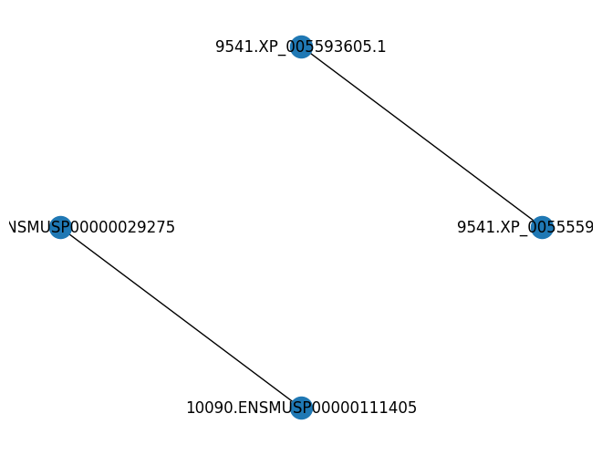
FLUTE offers the function of showing interactions within the same paper set as the input interaction file. Its inclusion of column “Paper IDs” allows such

[30]:

query = run_FLUTE.Query(db_user, db_password, db_host, db_name)
ints_same_pp = query.get_same_papers_ints(input_file, year_df)
ints_same_pp

[30]:

array([['9541.XP_005555920.1', '9541.XP_005593605.1', 'activation',
        'PMID018283119'],
       ['9541.XP_005593605.1', '9541.XP_005555920.1', 'activation',
        'PMID018283119'],
       ['10090.ENSMUSP00000029275', '10090.ENSMUSP00000111405',
        'activation', 'PMID018283119'],
       ['10090.ENSMUSP00000111405', '10090.ENSMUSP00000029275',
        'activation', 'PMID018283119']], dtype='<U50')

Our original interaction input was extracted very recently (or from papers without year information), thus there are just a handful of interactions that overlap with them

But we can still view these interactions in the same paper set in a network graph, thanks to networkx package

[31]:

G = nx.from_edgelist(ints_same_pp[:,:2])
nx.draw(G,pos=nx.circular_layout(G),with_labels=True)
plt.show()

Using FLUTE to query an individual protein

FLUTE also supports the extraction of list of papers that research on certain protein

[32]:

query_pro = "P00533,P03386"

[33]:

# get related papers
query = run_FLUTE.Query(db_user, db_password, db_host, db_name)
fq_list = query.get_related_papers(year_df, query_pro)

np.array(fq_list)

[33]:

array(['PMC1240052', 'PMC1540706', 'PMC1681463', 'PMC1702556',
       'PMC2132490', 'PMC2156182', 'PMC2225448', 'PMC2360392',
       'PMC2575782', 'PMC2742444', 'PMC2756567', 'PMC2824488',
       'PMC3088706', 'PMC3203921', 'PMC3234252', 'PMC3315809',
       'PMC3326441', 'PMC3398014', 'PMC3527276', 'PMC3569983',
       'PMC3730230', 'PMC3767783', 'PMC3952845', 'PMC3965010',
       'PMC4039121', 'PMC4039310', 'PMC4152746', 'PMC4213030',
       'PMC4226707', 'PMC4302072', 'PMC4390223', 'PMC4440518',
       'PMC4615268', 'PMC4724821', 'PMC4741629', 'PMC4791069',
       'PMC4826614', 'PMC5036527', 'PMC5117851', 'PMC5303889',
       'PMC5342422', 'PMC5432325', 'PMC5449203', 'PMC5461031',
       'PMC5531611', 'PMC5641085', 'PMC5648601', 'PMC5715073',
       'PMC5817799', 'PMC5935102', 'PMC5977112', 'PMC5992104',
       'PMC6053247', 'PMC6365915'], dtype='<U10')

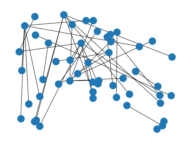
Use the function discussed above, interactions inside these papers can be extracted, these interactions co-occur with the inquired protein in the same literature and are of great research interest

[34]:

pd.DataFrame(fq_list, columns=['Paper IDs']).to_excel(output_path + '_query_' + query_pro + '.xlsx', index=False)
related_pp = query.get_same_papers_ints(output_path + '_query_' + query_pro + '.xlsx', year_df)

print("Number of interactions inside related_pp: ", len(related_pp))
related_pp[:15]

Number of interactions inside related_pp:  78

[34]:

array([['7227.FBpp0084623', '7227.FBpp0084626', 'binding',
        'PMID028515276'],
       ['7227.FBpp0084626', '7227.FBpp0084623', 'binding',
        'PMID028515276'],
       ['7227.FBpp0084626', '7227.FBpp0305095', 'binding',
        'PMID028515276'],
       ['7227.FBpp0305095', '7227.FBpp0084626', 'binding',
        'PMID028515276'],
       ['8364.ENSXETP00000021098', '8364.ENSXETP00000061006', 'binding',
        'PMID026344197'],
       ['8364.ENSXETP00000061006', '8364.ENSXETP00000021098', 'binding',
        'PMID026344197'],
       ['9606.ENSP00000175756', '9606.ENSP00000269571', 'ptmod',
        'PMID025081058'],
       ['9606.ENSP00000219070', '9606.ENSP00000301178', 'expression',
        'PMID027775700'],
       ['9606.ENSP00000261739', '9606.ENSP00000275493', 'binding',
        'PMID022298428'],
       ['9606.ENSP00000269571', '9606.ENSP00000175756', 'ptmod',
        'PMID025081058'],
       ['9606.ENSP00000275493', '9606.ENSP00000261739', 'binding',
        'PMID022298428'],
       ['9606.ENSP00000275493', '9606.ENSP00000301178', 'ptmod',
        'PMID027775700'],
       ['9606.ENSP00000275493', '9606.ENSP00000355396', 'binding',
        'PMID025353163'],
       ['9606.ENSP00000275493', '9606.ENSP00000368667', 'binding',
        'PMID028152297'],
       ['9606.ENSP00000275493', '9606.ENSP00000460823', 'binding',
        'PMID019798056']], dtype='<U50')

[35]:

# View these interactions in a networkx graph
G = nx.from_edgelist(related_pp[:,:2])
nx.draw(G,pos=nx.random_layout(G),with_labels=False)
plt.show()

Using FLUTE to find recent interactions

[36]:

# Map the input interaction file with its paper published year
df = pd.read_excel(input_file)
df = df.merge(year_df, left_on='Paper IDs', right_on='PMCID')
df['Year']=df['Year'].astype('int64')
df

[36]:

	Regulator Name	Regulator Type	Regulator Subtype	Regulator HGNC Symbol	Regulator Database	Regulator ID	Regulator Compartment	Regulator Compartment ID	Regulated Name	Regulated Type	...	Cell Type	Tissue Type	Organism	Score	Source	Statements	Paper IDs	Year	PMCID	PMID
0	CAR	Protein	NaN	NaN	NaN	P36575	NaN	NaN	tumor	Biological Process	...	cl:CL:0000084	NaN	uberon:UBERON:0002015	NaN	NaN	Anti-CAIX CAR T cells secreting anti-PD-L1 ant...	PMC5085160	2016	PMC5085160	PMID:27145284
1	CAR	Protein	NaN	NaN	NaN	P36575	NaN	NaN	ADCC	Biological Process	...	cl:CL:0000084 ++++ cl:CL:0001063	NaN	NaN	NaN	NaN	Moreover , anti-CAIX CAR T cells secreting the...	PMC5085160	2016	PMC5085160	PMID:27145284
2	IgG1 isoform	Other	NaN	NaN	NaN	UAZ496747312069736F666F726D	NaN	NaN	ADCC	Biological Process	...	cl:CL:0000084 ++++ cl:CL:0000623	NaN	NaN	NaN	NaN	For the anti-CAIX CAR T cells secreting anti-P...	PMC5085160	2016	PMC5085160	PMID:27145284
3	CAR	Protein	NaN	NaN	NaN	P36575	NaN	NaN	CAIX	Protein	...	cl:CL:0000084 ++++ cl:CL:0000623	NaN	NaN	NaN	NaN	The anti-CAIX CAR T cells only produced IL-2 a...	PMC5085160	2016	PMC5085160	PMID:27145284
4	CAIX	Protein	NaN	NaN	NaN	Q16790	NaN	NaN	CAR	Protein	...	cl:CL:0000084 ++++ cl:CL:0000623	NaN	NaN	NaN	NaN	The anti-CAIX CAR T cells only produced IL-2 a...	PMC5085160	2016	PMC5085160	PMID:27145284
...	...	...	...	...	...	...	...	...	...	...	...	...	...	...	...	...	...	...	...	...	...
3112	CD4	Protein	NaN	NaN	NaN	P01730	NaN	NaN	IL7	Protein	...	cl:CL:0000084	NaN	NaN	NaN	NaN	The percentage of CD4 CARGD2.28.OX40 ζ T cells...	PMC5980417	2018	PMC5980417	PMID:29872565
3113	ζ	Other	NaN	NaN	NaN	UAZCEB6	NaN	NaN	IL7	Protein	...	cl:CL:0000084	NaN	NaN	NaN	NaN	The percentage of CD4 CARGD2.28.OX40 ζ T cells...	PMC5980417	2018	PMC5980417	PMID:29872565
3114	CAR.GD2	Other	NaN	NaN	NaN	UAZ4341522E474432	NaN	NaN	proliferation	Biological Process	...	cl:CL:0000084 ++++ cl:CL:0000034 ++++ cl:CL:00...	NaN	NaN	NaN	NaN	These cytokines are known to enhance survival ...	PMC5980417	2018	PMC5980417	PMID:29872565
3115	ζ	Other	NaN	NaN	NaN	UAZCEB6	NaN	NaN	IL2	Protein	...	cl:CL:0000084 ++++ cl:CL:0000034 ++++ cl:CL:00...	NaN	NaN	NaN	NaN	After exposure to GD2 tumor cells , a higher q...	PMC5980417	2018	PMC5980417	PMID:29872565
3116	TGFB	bioprocess	NaN	NaN	NaN	D016212	NaN	NaN	FOXP3	Other	...	NaN	NaN	NaN	0.86	INDRA	AKT * impairs de novo Foxp3 induction by TGF-b...	PMC2275380	2008	PMC2275380	PMID:18283119

3117 rows × 31 columns

[37]:

binned_series = df["Year"].value_counts(bins=12, sort=False)

chart_data_binned = pd.DataFrame({
    "leftbin": binned_series.index.left,
    "rightbin": binned_series.index.right,
    "count": binned_series.values
})

chart_data_binned.loc[0, "leftbin"] = df["Year"].min()

quant_chart = alt.Chart(chart_data_binned).mark_bar(color="#fca5a5").encode(
    x = alt.X("leftbin", bin="binned", title="Year (binned)"),
    x2 = "rightbin",
    y = alt.Y("count")
).properties(
    width=500,
    height=200,
    title = 'Published Year Distribution of All Input Interactions (Unknown Removed)'

)

quant_chart

[37]:

[38]:

# Define a number of years
x = 5  # recent 5 years
df = df[df['Year'] >= time.localtime().tm_year - x].drop(columns=year_df.columns)

This DataFrame only contains recent (less than 5 years) interactions published at a known year. The number shrinks a lot compared to original input interaction file

This is useful if users want to exempt these interactions from filtering

[39]:

df

[39]:

	Regulator Name	Regulator Type	Regulator Subtype	Regulator HGNC Symbol	Regulator Database	Regulator ID	Regulator Compartment	Regulator Compartment ID	Regulated Name	Regulated Type	...	Mechanism	Site	Cell Line	Cell Type	Tissue Type	Organism	Score	Source	Statements	Paper IDs
13	UniCAR	Other	NaN	NaN	NaN	UAZ556E69434152	NaN	NaN	4-1BB	Protein	...	NONE	NaN	NaN	cl:CL:0000815 ++++ cl:CL:0001063	NaN	NaN	NaN	NaN	As shown in Figure 4 ( a ) ( middle panel ) , ...	PMC6685520
14	TCR-	Other	NaN	NaN	NaN	TCR	NaN	NaN	proliferation	Biological Process	...	NONE	NaN	NaN	cl:CL:0000815	NaN	NaN	NaN	NaN	To further support the aforementioned findings...	PMC6685520
15	luciferase	Protein	NaN	NaN	NaN	Q01158	NaN	NaN	tumor	Biological Process	...	NONE	NaN	NaN	cl:CL:0000815 ++++ cl:CL:0001063	NaN	NaN	NaN	NaN	In mice transplanted with UniCAR endowed Tconv...	PMC6685520
16	UniCAR	Other	NaN	NaN	NaN	UAZ556E69434152	Other	sl-0487	CD4 CD25 CD127	Other	...	NONE	NaN	NaN	cl:CL:0000084 ++++ cl:CL:0000815	NaN	NaN	NaN	NaN	To investigate responsiveness of UniCAR armed ...	PMC6685520
17	CD3	Other	NaN	NaN	NaN	CD3	NaN	NaN	T cell activation	Biological Process	...	NONE	NaN	NaN	cl:CL:0000084 ++++ cl:CL:0000236	NaN	NaN	NaN	NaN	Originally , first generation CARs were design...	PMC6685520
...	...	...	...	...	...	...	...	...	...	...	...	...	...	...	...	...	...	...	...	...	...
3085	mAb	Other	NaN	NaN	NaN	UAZ6D4162	Other	sl-0431	SHP-2	Protein	...	Phosphorylation	NaN	NaN	cl:CL:0000235 ++++ cl:CL:0000236 ++++ cl:CL:00...	NaN	NaN	NaN	NaN	Functionally , mAb targeting PD-L1 was able to...	PMC6558778
3086	PD-1	Protein	NaN	NaN	NaN	P18621.t	NaN	NaN	PD-L1	Protein	...	Transcription	NaN	cellosaurus:CVCL_1905	mesh:D015496 ++++ cl:CL:0000623 ++++ mesh:D018...	NaN	NaN	NaN	NaN	Furthermore , lenalidomide , an immunomodulato...	PMC6558778
3087	PD-L1	Protein	NaN	NaN	NaN	Q9NZQ7	Other	sl-0431	SHP-2	Protein	...	Phosphorylation	NaN	NaN	cl:CL:0000235 ++++ cl:CL:0000236 ++++ cl:CL:00...	NaN	NaN	NaN	NaN	Functionally , mAb targeting PD-L1 was able to...	PMC6558778
3088	mAb	Other	NaN	NaN	NaN	UAZ6D4162	Other	sl-0431	SHP-2	Protein	...	Phosphorylation	NaN	NaN	cl:CL:0000235 ++++ cl:CL:0000236 ++++ cl:CL:00...	NaN	NaN	NaN	NaN	Functionally , mAb targeting PD-L1 was able to...	PMC6558778
3089	CD4	Protein	NaN	NaN	NaN	P01730	NaN	NaN	transmembrane protein	Protein	...	Transcription	NaN	NaN	cl:CL:0000911 ++++ cl:CL:0000623 ++++ cl:CL:00...	NaN	NaN	NaN	NaN	Lymphocyte activation gene-3 ( LAG-3 ) is a tr...	PMC6558778

1367 rows × 28 columns

Using FLUTE to find duplicate interactions

[40]:

df = pd.read_excel(input_file)

columns_to_check = ['Regulated ID', 'Regulator ID', 'Paper IDs']
duplicates = df[df.duplicated(subset=columns_to_check, keep=False)]
duplicate_counts = duplicates.groupby(columns_to_check).size().reset_index(name='Occurrence')

This DataFrame contains the duplicated interactions (based on Regulated ID, Regulator ID, Paper IDs) of the original input file and their occurrences.

This is helpful when user wants to only keep unique interactions

[41]:

duplicate_counts.sort_values(by='Occurrence', ascending=False)

[41]:

	Regulated ID	Regulator ID	Paper IDs	Occurrence
462	Q9NZQ7	Q9NZQ7.t	PMC10098269	8
278	P18621	P31947	PMC8614004	5
319	P29597	P18031	PMC8904293	5
209	P01375	P05231.s	PMC8018404	4
458	Q9NZQ7	P31947	PMC8614004	4
...	...	...	...	...
175	Interferon	P36575	PMC6174845	2
174	Interferon	P01730	PMC3654581	2
173	Interferon	CD8	PMC3654581	2
172	IPR011584	P36575:[SubstitutionMutant]	PMC9853244	2
532	p38	CHEBI:90705	PMC10098269	2

533 rows × 4 columns

From this table, we might have insights into what species are elaboratively studied

[42]:

topk_series = duplicate_counts["Regulated ID"].value_counts().iloc[:5]
total_count = len(duplicate_counts)
topk_df = pd.DataFrame({"Regulated ID": topk_series.index, 'percentage': (topk_series / total_count) * 100})

# Create the bar chart
upper = alt.Chart(topk_df).mark_bar(color="#bae6fd").encode(
    x=alt.X("percentage", title="Percentage of Top 5 Repeated Regulated IDs"),
    y=alt.Y("Regulated ID:N", sort="-x", title="")
).properties(
    width=500,
    height=200
)

topk_series = duplicate_counts["Regulator ID"].value_counts().iloc[:5]
total_count = len(duplicate_counts)
topk_df = pd.DataFrame({"Regulator ID": topk_series.index, 'percentage': (topk_series / total_count) * 100})

# Create the bar chart
lower = alt.Chart(topk_df).mark_bar(color="#fdd1ba").encode(
    x=alt.X("percentage", title="Percentage of Top 5 Repeated Regulator IDs").scale(domain=[0, 12]),
    y=alt.Y("Regulator ID:N", sort="-x", title="")
).properties(
    width=500,
    height=200
)

alt.vconcat(upper, lower)

[42]: